Today’s topic is AlexNet from NIPS 2012. AlexNet is the winner of ImageNet Large Scale Visual Recognition Challenge (ILSVRC) 2012.
Prior to ILSVRC 2012, competitors mostly used feature engineering techniques combined with a classifier (i.e SVM).
AlexNet marked a breakthrough in deep learning where a CNN was used to reduce the error rate in ILSVRC 2012 substantially and achieve the first place of the ILSVRC competition.
The highlights of this paper: - Breakthrough in Deep Learning using CNN for image classification. - Multi-GPUs - Use ReLU - Use Dropout
Outline
AlexNet
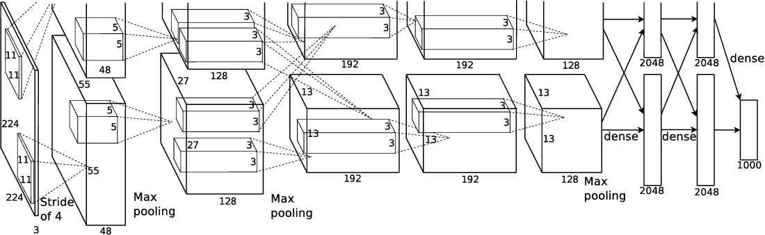
Architecture
AlexNet contains five convolutional and three fully-connected layers. The output of the last fully-connected layer is sent to a 1000-way softmax layer which correspondes to 1000 class labels in the ImageNet dataset.
The network takes between five and six days to train on two GTX 580 GPUs with 3GB memory.
Here is a summary of AlexNet layers:
| Layer | Components |
|---|---|
| Input | 224 x 224 x 3 Images |
| 1 | Conv 96 kernels of size 11 x 11 x 3, stride 4, padding 0 ReLU Local Response Normalization 55 x 55 x 96 features maps Overlapping Max Pooling, size 3 x 3, stride 2 27 x 27 x 96 features maps |
| 2 | Conv 256 kernels of size 5 x 5 x 48, stride 1, padding 2 ReLU Local Response Normalization 27 x 27 x 256 features maps Overlapping Max Pooling, size 3 x 3, stride 2 13 x 13 x 256 features maps |
| 3 | Conv 384 kernels of size 3 x 3 x 256, stride 1, padding 1 ReLU 13 x 13 x 384 features maps |
| 4 | Conv 384 kernels of size 3 x 3 x 192, stride 1, padding 1 ReLU 13 x 13 x 384 features maps |
| 5 | Conv 256 kernels of size 5 x 5 x 192, stride 1, padding 2 ReLU Local Response Normalization 13 x 13 x 256 features maps Overlapping Max Pooling, size 3 x 3, stride 2 6 x 6 x 256 features maps |
| 6 | Fully Connected Layer of 4096 neurons |
| 7 | Fully Connected Layer of 4096 neurons |
| 8 | Fully Connected Layer of 1000 neurons |
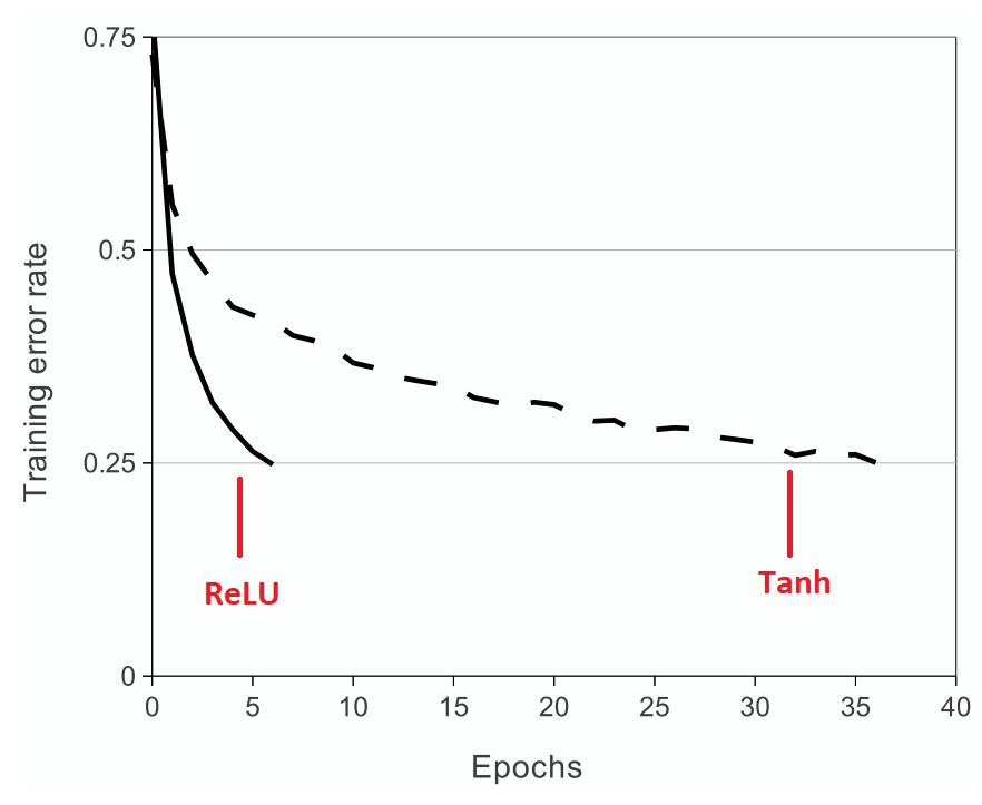
ReLU nonlinearity
Before AlexNet, sigmoid and tanh were usually used as activations which are saturating nonlinearities. AlexNet uses Rectified Linear Units (ReLUs) activations which are non-saturating nonlinearity.
The formula of ReLU is:
$$f(x) = max(0, x)$$
The benefits of ReLU are:
- Avoid vanishing gradients for positive values.
- More computationally efficient to compute than
sigmoidandtanh. - Better convergence performance than
sigmoidandtanh.
Multi-GPUs
We can see that the architecture is splitted into two parallel parts. In Alexnet, 1.2 million training parameters are too big to fit into the NVIDIA GTX 580 GPU with 3GB of memory. Therefore, the author spread the network across two GPUs.
In this paper, the usage of two GPUs is due to memory limitation, not for distributed training as in current years.
Nowaday, the NVIDIA GPUs are large enough to handle this tasks. Therefore, the implementation will now split the network into two parts.
Overlapping Pooling
Traditionally, the neighbor neurons by adjacent pooling units do not overlap. In this paper, the author uses overlapping max pooling of size 3 x 3 with stride 2.
This scheme reduces the top-1 and top-5 error rates by 0.4% and 0.3%, respectively, as compared to max pooling of size 2 x 2 with stride 2.
Local Response Normalization
Local Response Normalization (LRN) is used in AlexNet to help with generalization.
The formula of Local Response Normalization (LRN) is:
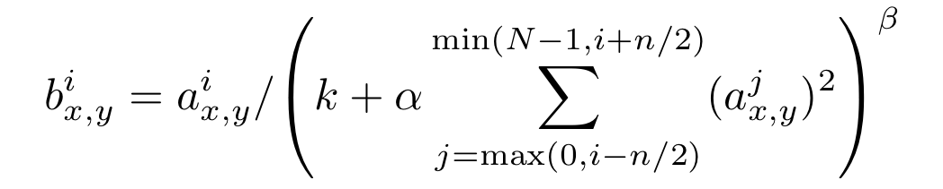
where:
- $a$: activation of a neuron
- $i$: $i$-th kernel
- $N$: total number of kernels
- $k$, $n$, $\alpha$, $\beta$: hyper parameters whose values are determined using a validation set; $k = 2$, $n = 5$, $\alpha = 10^{-4}$, $\beta = 0.75$
LRN reduces the top-1 and top-5 error rates by 1.4% and 1.2%.
In 2014, Karen Simonyan et al (VGGNet) shows that LRN does not improve the performance on ILSVRC dataset but leads to increased memory and computation time.
Nowdays, batch normalization is used instead of LRN.
Reduce Overfitting
DropOut
AlexNet uses a regularization technique called DropOut which will randomly set the output of each hidden neuron to zero with the probability of $p = 0.5$. Those dropped out neurons do not contribute to forward and backward passes.
DropOut reduces complex co-adaptaions of neurons, since a neuron cannot rely on the presence of particular other neurons.
Traditionally, in test time, we will need to multiply the outputs by $p = 0.5$ so that the response will be the same as training time. In implementation, it is common to rescale the remainder neurons, which are not dropped out, by dividing by $(1 - p)$ in training time. Therefore, we don’t need to scale in test time.
Data Augmentation
AlexNet uses two forms of data augmentation.
- First: translations and horizontal reflections: Extract random
224 x 224patches (and reflections) from256 x 256images. This technique increases the size of training set by a factor of2048.- Extract 224 x 224 from 256 x 256 images: $(256 - 224) * (225 - 224) = 1024$
- Horizontal reflections: $1024 * 2 = 2048$
- Second: altering the intensities of RGB channels: perform PCA on the set of RGB pixel values throughout the training set. Then, use the eigenvalues and eigenvectors to manipulate the pixel intensities. Eigenvalues are selected once for entire pixels of an particular image.
Other details
- Train with Stochastic Gradient Descent with:
- Batch size: 128
- Momentum: 0.9
- Weight Decay: 0.0005
- Initialize the weights in each layer from a zero-mean Gaussian distribution with std 0.01.
- Bias: Initialize 1 for 2nd, 4th, 5th conv layers and fully-connected layers. Initialize 0 for remaining layers.
- Learning rate: 0.01. Equal learning rate for all layers and diving by 10 when validation error stopped improving.
- Train roughly 90 cycles with 1.2 million training images, which took 5 to 6 days on two NVIDIA GTX 580 3GB GPUs.
Results
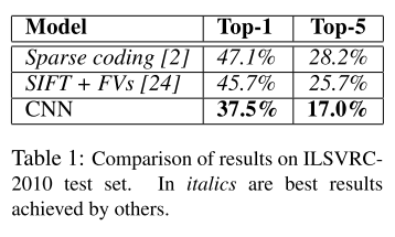
- Results on ILSVRC-2010: top-1 and top-5 test set error rates of 37.5% and 17.0%. Sparse coding and SIFT + FVs are best performances prior AlexNet.
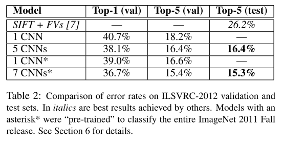
- Results on ILSVRC-2012:
Implementations
In this section, we will review the implementation of AlexNet in Pytorch. First, we will take a look at the AlexNet from pytorch/vision repository. This implementation is different in term of conv features and lacks of Local Response Normalization. Second, we will look at an implementation that matches with the paper.
AlexNet from torchvision
This is AlexNet implementation from pytorch/torchvision.
Note:
- The number of nn.Conv2d doesn’t match with the original paper.
- This model uses
nn.AdaptiveAvgPool2dto allow the model to process images with arbitrary image size. PR #746 - This model doesn’t use Local Response Normalization as described in the original paper.
- This model is implemented in Jan 2017 with pretrained model.
- PyTorch’s Local Response Normalization layer is implemented in Jan 2018. PR #4667
AlexNet with LRN
This is the implementation of AlexNet which is modified from Jeicaoyu’s AlexNet.
Note:
- The number of Conv2d filters now matches with the original paper.
- Use PyTorch’s Local Response Normalization layer which is implemented in Jan 2018. PR #4667
- This is for educational purpose only. We don’t have pretrained weights for this model.
Reference
[NIPS 2012] [AlexNet] ImageNet Classification with Deep Convolutional Neural Networks.
[2015 ICLR] [VGGNet] Very Deep Convolutional Networks for Large-Scale Image Recognition
My Reviews
- Image Classification: [NIPS 2012] AlexNet
- Image Segmentation: [CVPR 2019] Pose2Seg
- Pose Estimation: [CVPR 2017] OpenPose
- Pose Tracking: [CVPR 2019] STAF